Periodogram Recipe: Examining Variable Star Data From an Input File
User Guide
Using the Service:The following procedure demonstrates how to examine variable star data from a user-uploaded input file. There is another procedure that describes how to calculate a periodogram from a Kepler time series that is stored in the Exoplanet Archive.
The example we've chosen is a Delta Scuti star with dominant frequencies below the long cadence Nyquist frequency. Running the Periodogram service on long cadence data gives you an aliased period; using the short cadence data recovers the correct period.
- First, download the following input files to your computer:
- deltaScutiLightcurveLC.txt (Long Cadence)
- deltaScutiLightcurveSC.txt (Short Cadence)
- Go to the Periodogram home page and upload the long cadence (deltaScutiLightcurveLC.txt) file in the Input File Options pane of the Periodogram Inputs tab.
- Click Choose File and browse to your local copy.
- Click Upload
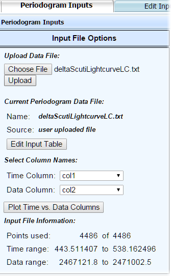
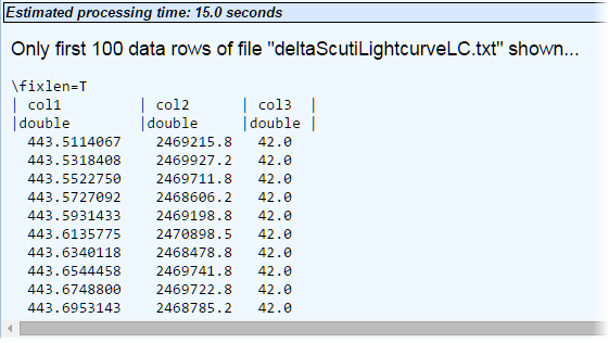
- Briefly check your data in the preview pane at bottom of the Periodogram Inputs tab to ensure they loaded correctly.
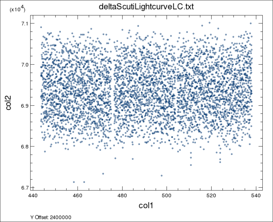
- Click the Plot Input tab and then the Plot Time vs. Data Columns button. This action plots the time vs. data columns and provides a preview plot of your input data. Note that the scatter along the Y-axis looks as expected, and there are no visible periodicities. Compare your result:
- Return to Periodogram Inputs tab and click Calculate Periodogram. Note that for this example, we are using the default algorithm and period settings and output options.
- The result displays on the Results tab. Note that there are three significant peaks listed in the Table of Peaks to the right. Compare your result:
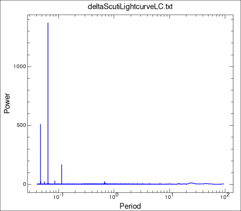
- Click View for the Rank 1 curve listed in the table, which opens a new browser tab and shows the periodogram for the highest-power period.
- Return to your web browser's tab (labeled deltaScutiLightcurveLC.txt) and click the Periodogram Inputs tab to upload the short cadence input file:
- Click Choose File and browse to your local copy of deltaScutiLightcurveSC.txt.
- Click Upload.
- As you did in step 3, briefly check your data in the preview pane at bottom of the Periodogram Inputs tab. (Make sure you click Upload so you're not viewing the long cadence file.)
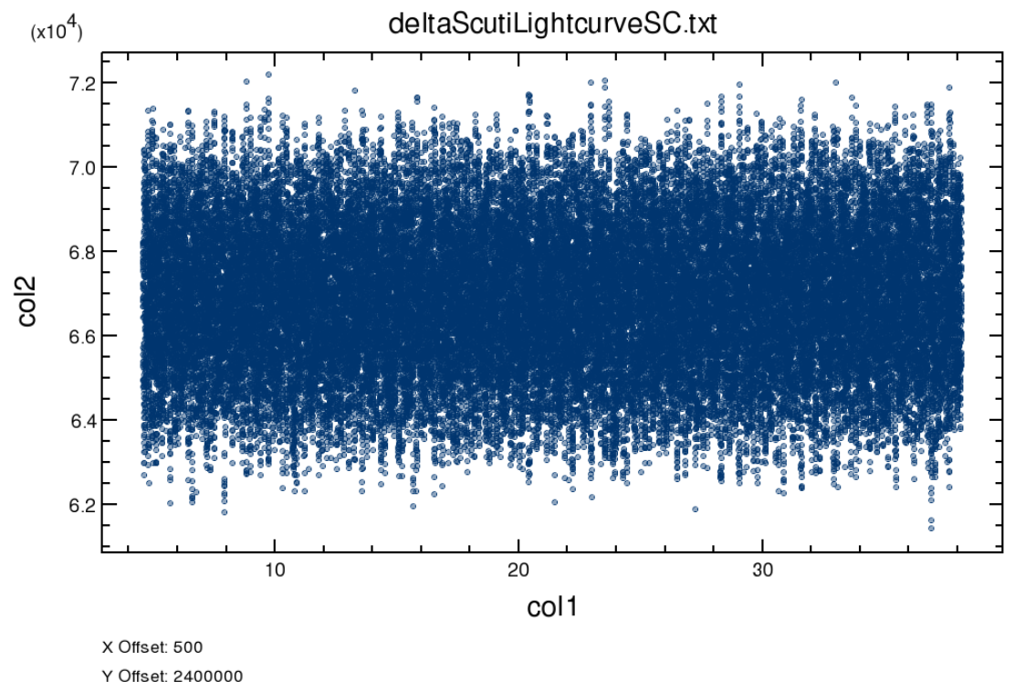
- As you did in step 4, click the Plot Input tab and then the Plot Time vs. Data Columns button to preview the plot. Compare your result:
- Return to the Periodogram Inputs tab and click the Calculate Periodogram button. Wait for the job to process. When prompted, view the periodogram on the Results tab. Compare your result:
- As you did in step 7, click View for the Rank 1 curve listed in the table, which opens a new browser tab and shows the periodogram for the highest-power period. Compare your result:
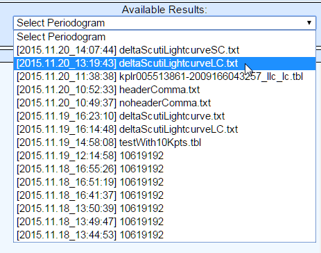
- To compare the short cadence and long cadence periodograms, return to the Periodogram Inputs tab and select the deltaScutiLightcurveLC.txt session from the Available Results: drop-down menu (the session name is preceded by a timestamp). Note that this is the same way you would return to your short cadence periodogram results.

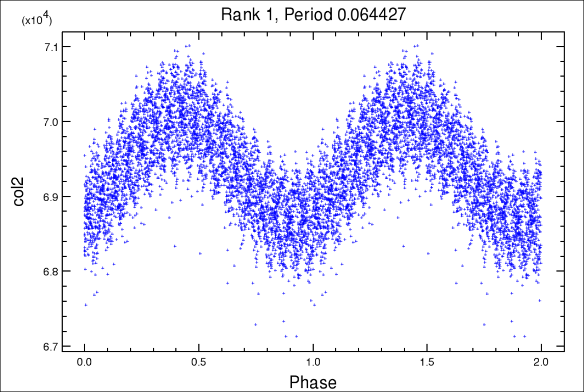
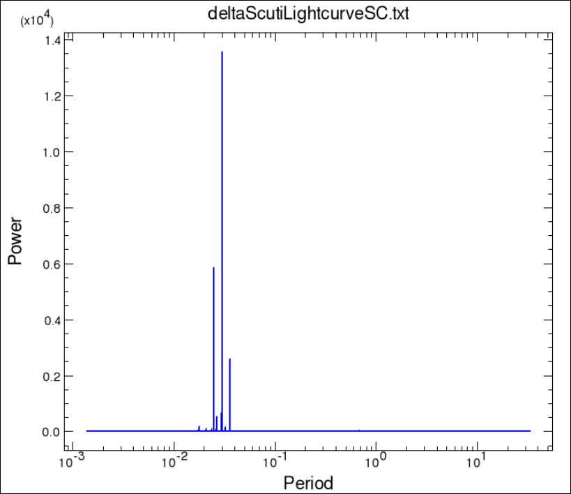
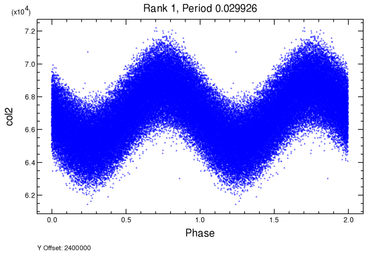
In the short cadence periodogram, you can see the same three peaks as you did in the long cadence periodogram, but note that the periods in the Table of Peaks are different periods from the long cadence results. The short cadence results are the correct periods; the long cadence results were an alias of these results.
Last update: 26 April 2018