Algorithms

The algorithms currently implemented focomputing periodograms from light curves are Lomb-Scargle (Scargle 1982), Box-fitting Least Squares or "BLS" (Kovacs et al. 2002), and Plavchan (Plavchan et al. 2008).

Skip to a section:

Lomb-Scargle
Box-fitting Least Squares (BLS)
Plavchan

---

Lomb-Scargle

How it works

The Lomb-Scargle (L-S) algorithm (Scargle, 1982) is a variation of the Discrete Fourier Transform (DFT), in which a time series is decomposed into a linear combination of sinusoidal functions. The basis of sinusoidal functions transforms the data from the time domain to the frequency domain. DFT techniques often assume evenly spaced data points in the time series, but this is rarely the case with astrophysical time-series data. Scargle has derived a formula for transform coefficients that is similar to the DFT in the limit of evenly spaced observations. In addition, an adjustment of the values used to calculate the transform coefficients makes the transform invariant to time shifts.

How to Use the Algorithm

The Lomb-Scargle periodogram is optimized to identify sinusoidal-shaped periodic signals in time-series data. Particular applications include radial velocity data and searches for pulsating variable stars. L-S is not optimal for detecting signals from transiting exoplanets, where the shape of the periodic light curve is not sinusoidal.

N	number of points in the input file
df	step size in frequency space
dp	step size in period space
p(i)	output period value

Statistical Distribution

In the NASA Exoplanet Archive's implementation, the periodogram power is normalized by the inverse of the variance of the original signal data values. Horne and Baliunas (Horne, 1986) showed that this scaled power has an exponential distribution for Gaussian noise data values and a large number of observations N_obs. The probability, p, of observing a power less than or equal to P₀ in one sample when the time series is a noise signal is then given by:

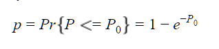
The probability of seeing at least one sample exceeding this value is then given by

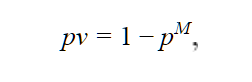
where M is the number of periods sampled.

The above expression is invalid in the limit of a small number of observations, N_obs. When N_obs is less than 50, the following formula is applied as in Zechmeister and Kürster (2009):

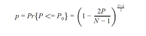
and, again

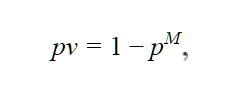
where M is now the number of independent frequencies. The theoretical number of independent frequencies for a given data set lies between N and N*(N-1)/2 (or N choose 2). The effective number of independent frequencies is approximately equal to

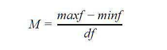
where df is the width (in frequency) of a peak (Zechmeister and Kürster, 2009) that is defined as the width of the top peak in the periodogram. The beginning and ending points of a peak are defined as the frequencies at which the power is half of the peak's maximum.

References

Horne, J.H., Baliunas, S.L. "A prescription for period analysis of unevenly sampled time series." Astrophysical Journal, 302:757-763 (1986) Abstract

Scargle, J.D. "Studies in Astronomical Time Series Analysis II: Statistical Aspects of Spectral Analysis of Unevenly Spaced Data." Astrophysical Journal, 263:835-853 (1982) Abstract

Zechmeister, M., Kürster, M. "The Generalised Lomb-Scargle Periodogram. A new Formalism for the Floating-mean and Keplerian Periodograms." Astronomy and Astrophysics, 496:577-584 (2009) Abstract

Box-fitting Least Squares (BLS)

How it works

The Box-fitting Least Squares (BLS) algorithm (Kovacs et al., 2002) fits the input time series to periodic "box"-shaped functions, rather than decomposing it into sinusoids as with the L-S algorithm. A box-shaped function consists of the superposition of two step functions with equal amplitude but opposite sign, and offset in time. A periodic box-shaped function alternates between a “low” and a “high” state, with a fixed fraction and phase of each periodic cycle in a given state.

Periodic box-shaped functions represent the behavior of a light curve during a transit better than sines and cosines; they are flat except for a repeated periodic dip in brightness that lasts, typically, for less than 10 percent of the total period. In the BLS algorithm, the signal is assumed to take on a "low" value for some fraction of the period and a "high" value for the remainder. Periodic box-shaped functions were chosen as a set of basis functions instead of sinusoids, because the typical transit light curve, when decomposed into Fourier frequency space, does not have a dominant frequency term. A periodic box-shaped functions requires many additive Fourier components. In order to detect transits, it is better to choose a set of basis functions that require only one term to generate a simple model light curve for the transit.

To determine the fit of these periodic box-shaped functions to the signal, consider a set of candidate periods. For each candidate period P, a time-series is "folded" to the period: for each data point i and time t_i, and there is a corresponding phase given by the formula phase_i = (t_i modulo P) / P. All data points are then placed into phase bins. The algorithm then considers various ranges of bins based on the input minimum and maximum fraction of a period that may be spent in transit, and identifies the best bin range to designate as the "low" state. The best least squares fit and relative amplitude of the "low" state for a candidate period determines the periodogram "power."

Adjustable Algorithm Parameters

• Number of bins - The BLS algorithm relies on binning data points and the number of bins may be specified as an input parameter. The goal is to choose the number of bins to achieve a balance between having a reasonable number of points in each bin and partitioning the phased time series into a reasonable number of pieces. "Reasonable" in each case depends on the number of points in your light curve; 50 bins is a typical number to use for ground-based transit surveys with a few thousand data points.


• Fraction of period in transit - The BLS algorithm hypothesizes that some fraction of the period will be spent in the "low" state and the remainder in the "high" state. You may specify the minimum and maximum allowable fraction of the period spent in the low state.

How to Use the Algorithm

The BLS periodogram is optimized to identify "box" or transit-shaped periodic signals in time-series data. Particular applications include searches for transiting exoplanets or detached eclipsing binaries. BLS is not optimal for detecting signals from pulsating variables or radial velocity exoplanets, where the shape of the time-series data variations is sinusoidal.

Statistical Distribution

The calculated periodogram distribution of power values for the BLS algorithm for a given time series is described very well by a normal (Gaussian) distribution. The NASA Exoplanet Archive measures the mean and standard deviation of the calculated periodogram values, and from this calculates the p-values, as is consistent with the literature. For large-amplitude variations or long-term trends, the resulting p-values may not be reliable, since these variations may alter the distribution of periodogram values from the idealized normal distribution.

References

Kovacs, G., Zucker, S. and Mazeh, T. "A box-fitting algorithm in the search for periodic transits." A&A 391:369-377 (2002) Abstract

Plavchan

How it works

The Plavchan periodogram (Plavchan et al., 2008) is similar to a binless variation of the "phase dispersion minimization" (PDM) algorithm (Stellingwerf, 1978). In this method, the "basis" of periodic curves is computed directly from the data. As in the BLS method, the time series is folded to the candidate period. A dynamical prior is generated by box-car smoothing the phased time series. The difference between the data and the prior is squared and summed over a worst-fit subset of the data. When a suitable period is found, the sum of the squared residuals from the smoothed curve will be minimized. If no signal is present, the minimum sum of squared errors will come from the model of no variability (i.e., data values = constant). This is used as the normalization. Periodogram power is defined as the normalization divided by the sum of squared residuals to the smoothed curve. It will be greater than one if the assumption of no variability is improved upon.

• Number of outliers - The "number of outliers" parameter allows adjustment of the Plavchan power calculation. When comparing the time series to the dynamical prior, computation may be restricted to the N worst-fitting data points. The worst-fit data points may change for different candidate periods, as the prior also changes. This improves sensitivity in low signal-to-noise searches.


• Phase-smoothing box size - The phase smoothing-box parameter specifies the width of the phase box over which to average the time-series data to compute the dynamical prior. A value of 0.05 is typical for ground-based transit surveys with a few thousand data points.

How to Use the Algorithm

Since the priors are dynamically generated from the data, the Plavchan algorithm can detect sinusoidal variations and box-shaped periodic functions equally well. It is useful to detect periodic time-series shapes that are not well described by the assumptions of other algorithms, for example: contact Algol eclipsing binaries, saw-toothed shaped light curves, and large eccentricity radial velocity curves. This algorithm is more computationally intensive than the L-S and BLS algorithms.

Statistical Distribution

The calculated periodogram distribution of power values for a given time-series is very well-described by a log-normal (log-Gaussian) distribution. See this example:

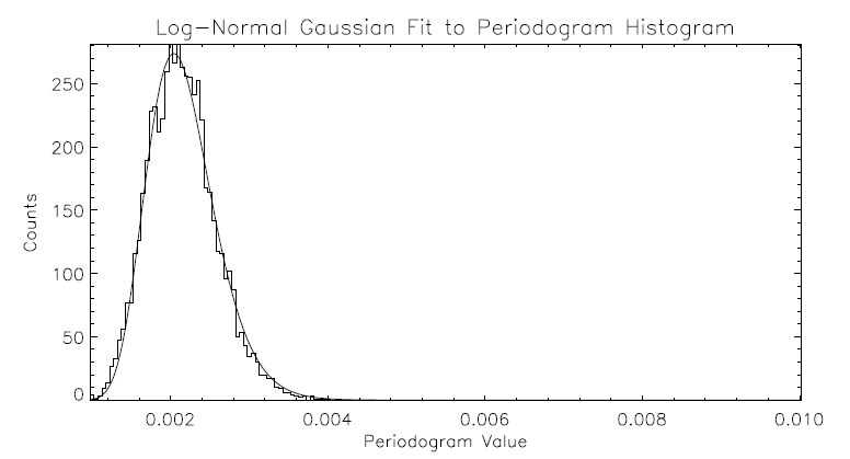
Note: The Plavchan algorithm is particularly sensitive to detecting periodogram peaks at integer multiples of the fundamental period. For extremely high signal-to-noise periodic variability signals, the distribution of periodogram values can deviate from the assumed log-normal distribution as many peaks are detected. This can in turn invalidate the p-value computation.

References

Plavchan, P., Jura, M., Kirkpatrick, J. D., Cutri, R.M., and Gallagher, S.C. "Near-Infrared Variability in the 2MASS Calibration Fields: A Search for Planetary Tranist Candidates." ApJS 175:191-228 (2008) Abstract

Stellingwerf, R. F. "Period Determination Using Phase Dispersion Minimization." Astrophysical Journal, 224:953-960 (1978) Abstract

Last update: 26 April 2018