EXOFAST Recipe: Run a Simple Fit
Documentation
Using the Service:- Accessing EXOFAST
- Overview of the Inputs Tab
- Accepted Input File Formats:
- Editing and Plotting Input Files
- Input Parameters and Options
- Output Parameters and Products
- Accessing Previous Results
- Usage Tips and Troubleshooting
Recipe: Run a Simple Fit
The following walk-through uses a known confirmed planet, HD 17156 b, to demonstrate the basic steps involved with running the EXOFAST interface, fitting both RV and transit data simultaneously. There is also a more advanced walk-through that serves as a tutorial for running a more complex fit.
Step 1: Load Transit Photometry Data
- Go to EXOFAST home, or click the red Start New Session button if you already have it open. You should see the EXOFAST Inputs tab as your default view.
- Download this transit photometry data file (26 KB), which is a light curve from Gillon et al. 2008 in IPAC table format from the NASA Exoplanet Archive. This light curve is already normalized and contains one complete, clean transit, with no unnecessary data.
- For Band in the Transit File Options pane, select B.
- In the same pane, click Browse and select the file you downloaded, then click Upload to send the file to the interface. Notice that details of the uploaded file display in the pane.
- Scroll down to the bottom half of the interface and look at the file upload preview pane. Notice the first 100 rows of your uploaded file displays. This step is to ensure you selected the correct file.
- Scroll back up to the Transit File Options pane and notice the first three columns, BJD, Normalized_Flux, and Normalized_Flux_Uncertainty are already selected for the time, flux, and error columns, respectively.
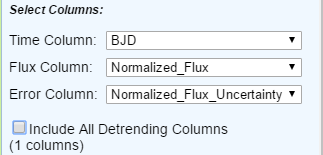
- Uncheck the Include All Detrending Columns box. Although there is one additional data column in the file, there are no detrending data.
- Click the Plot Data vs. Time button to preview a plot of the photometry data you've uploaded on the Plot Transit File tab.
Tip: Click Edit Input Table to view the parsed data table, or go directly to the Edit Transit File tab. On this tab, you could sort and filter data as you would with any of the archive's interactive tables, though this is not necessary for our example.
When finished, return to the EXOFAST Inputs tab.
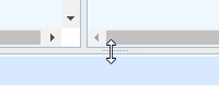
Tip: You can resize any of the panes by hovering the cursor over a border until it changes to two arrows, then dragging and dropping to a new location.
Step 2: Load Radial Velocity Data
Radial velocity files in the archive usually need no additional preparation and can be directly loaded into EXOFAST, rather than using the Upload option. For this example, we will use NASA Exoplanet Archive data.
- On the EXOFAST Inputs tab, go to the Radial Velocity File Options pane and enter HD 17156 for Host.
- From the Source drop-down list, select the RV curve HIRES-10m Keck/Winn et al. 2009. This file has plenty of data points over a long time-baseline, and very good signal-to-noise ratio. As you did for the transit photometry file upload, you may scroll to the bottom of the tab for a quick-look preview of the file's contents.
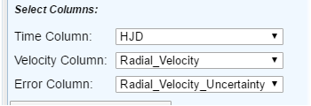
- Notice that EXOFAST has automatically designated HJD, Radial_Velocity and Radial_Velocity_Uncertainty as the Time, Velocity, and Error columns, respectively.
Step 3: Set Period and Setting Inputs
- Go to the Period and Setting Inputs pane and notice the default values are auto-populated for Minimum Period, Maximum Period, and # RV Periodogram Peaks. Leave these values; they represent the range and number of periods that can be explored during RV pre-fitting.
- Use the default setting for the rest of the options in this pane, which are:
- Force Circular Orbit is unchecked: This planet is on a very eccentric orbit, so a circular fit will not work.
- Chi-squared radio button is selected. We will first run a simple χ2 fit.
- Fit Slope to RV is unchecked.
- Kepler Long Cadence is unchecked.
Step 4: Set Prior and Prior Width Inputs
- Go to the Prior and Prior Width Inputs pane and enter HD 17156 b for Planet Name.
- Click Load Priors and Widths to auto-populate the input boxes with the available default parameters taken directly from the archive's Confirmed Planets Table. These will be used as initial starting points for the chi-squared fitting. We will use them as priors for an MCMC fit later in this walk-through.
- The default set of parameters in the archive does not include metallicity, which is required to run EXOFAST; the metallicity prior entries should now be highlighted as a warning.
However, if we look up the Confirmed Planet Overview Page for HD 17156 b in the archive, we see there are other (non-default) parameter sets in the archive that include metallicity, and they all roughly agree. We will use those values for our example: enter 0.24 for the prior value and 0.03 for the prior width.

Tip: Read our FAQ for an explanation of default parameters in the archive.
Step 5: Run EXOFAST and Review Results
- Enter HD17156b-chi as the Run Name.
- Click Run EXOFAST at the bottom-left corner of the screen and wait a few minutes for the program to complete the calculations. When the run finishes, the Results tab will automatically display containing all of the outputs of the calculations, including plots of the RV and transit fits, best-fit model parameters, links to all output data products, and a summary of all input parameters.
Tip: See the EXOFAST Output Parameters and Products page of this user guide for a detailed description of what you may find on the Results tab.

Step 6: Run a Full MCMC Calculation
Once you have reviewed the χ2 fit, you can use the same data sets to run an MCMC analysis. To do this:
- Return to the Inputs tab and select MCMC in the Period and Setting Inputs pane.
- Enter HD17156b-mcmc as the Run Name.
- Click Run EXOFAST. This run should typically take 10-20 minutes to process, depending on the current server load and how many MCMC steps are needed before EXOFAST determines the chains have converged. It is very like you will be given the option to receive an email notification when the calculation is complete.
When the run is finished, the Results tab will display with MCMC-specific outputs, including a table of median model parameter values, along with their 68% confidence intervals, plots of covariances and posterior probability distributions, etc. If you compare with the HD 17156 Planet Host Overview page, you should find the EXOFAST output parameters are very comparable with previously published values from the literature.

You can return to these calculations within the next four days by clicking the Available Results drop-down menu at the bottom-right area of the EXOFAST Inputs tab and selecting either of the runs you created (i.e HD17156b-chi or HD17156b-mcmc).
«Previous Usage Tips and Troubleshooting Recipe: Run an Advanced Fit Next »
Last update: 19 July 2017