Transit Algorithms
User Guide
Using the Service:Skip to a Section:
The EphemerisPlanet Model Parameters
Transit Visibility
Rise/Set Times
Observability Statistics
Transit Depth
How the Ephemerides are Calculated
The calculation of the transit ephemerides is based on an algorithm developed by Greg Laughlin of UC Santa Cruz.
The algorithm is linear and comprised of a small number of steps:
- The data are retrieved from the NASA Exoplanet Archive's databases, and may be superseded by any parameters input into the Custom Parameters interface. These parameters include planetary and stellar data, and information on transit properties, for example:
- Planet name (e.g., "55 Cnc b")
- Orbital period and uncertainty
- Epoch of periastron passage and uncertainty
- Planet orbital eccentricity
- Longitude (or strictly, argument) of periastron
- Stellar mass (for model)
- Planet radius
- Stellar radius
- Right ascension and declination
- Transit duration (if known) and uncertainty
- Transit midpoint and uncertainty
- An ephemeris may be computed by one of two means: through knowledge of the planet's orbital elements and planetary and stellar radii; or via a known transit duration and midpoint epoch.
- Once the necessary inputs are collected, the algorithm determines whether any parameters are missing. If using the orbital elements, two of these parameters, the planetary radius and semi-major axis, may be produced via planetary models, if missing; see the section below on Planet Model Parameters for more. If other parameters are unavailable, the service will notify you.
- Next, the ephemeris is computed:
- Transit Ephemeris Method: Since the transit midpoint is known, the algorithm simply iterates over the period, including uncertainties, such that
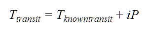
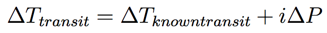
where Ttransit and Tknowntransit are the times of the predicted and known transit midpoints, respectively, i is an integer, and P is the orbital period. The beginning and ending of the transit window are computed, both with and without padding for propagated uncertainties in the period, transit duration and transit midpoint. Results are reported as 1σ Event Window Start and 1σ Event Window End (including uncertainty padding), and Event Ingress and Event Egress (excluding uncertainty padding), in the Results table. The 1σ window start and end represent the earliest and latest times, respectively, that the ingress and egress are predicted to occur, taking into account the reported sources of error. For example, for the beginning of the window:

where Δ is used to indicate uncertainties in a quantity (i.e., ΔP is the period uncertainty, and ΔTmidpoint is the transit midpoint uncertainty). We also propagate an uncertainty on the predicted transit midpoint. The uncertainty on the transit midpoint is calculated as:
- Orbital Elements: The planet's orbital position is determined by finding the time since periastron passage. The orbital elements algorithm assumes that argument (or 'longitude') of periastron, ω, refers to that of the star in its reflex orbit, rather than that of the planet; we also assume that positive radial velocity indicates motion along the line of sight moving away from the observer. Note that there is a mix of conventions in the literature, and it is not always clear which convention is used. Values in the Exoplanet Archive tables are as-published, and where a different convention is used by authors, the ephemerides predicted with this method may be substantially incorrect (for example, for a circular orbit, predictions will be off by half the orbital period). Results of this algorithm should therefore be treated with caution!
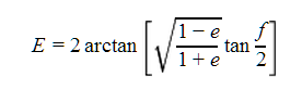
- Given the longitude (argument) of periastron, ω, compute the true anomaly ƒ = π/2 - ω, assuming that the true longitude Θ = π/2.
- Compute the eccentric anomaly E, given the eccentricity, e:
- Finally, compute the time since periastron passage,
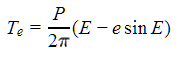 where P is the period. Note that the term in parentheses is Kepler's equation, which has been substituted for the mean anomaly.
- Compute the transit duration:
- Compute the change in true anomaly due to the transit,
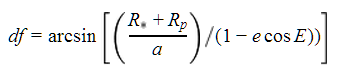
- Compute the adjusted true anomaly, ƒ + dƒ.
- Compute the adjusted eccentric anomaly Ε, as in the first equation in this section.
- Compute the transit duration, tT = PM/π where M is the mean anomaly, M= Ε - e sinΕ.
- The time of central transit is computed by iterating over orbital periods, given the time of periastron passage, Tperi , and the time since passage Te, such that
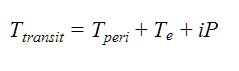
where i is the loop index.
In order to include padding for uncertainties in the start and end of the transit window, the differences from periastron passage time are first first computed from the orbital elements: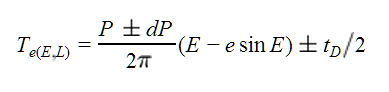
And then the start and end times of the window are found from:
As in the Transit Ephemeris method above, these times are reported as the 1σ Event Window Start and 1σ Event Window End in the output table on the Results tab, and represent the earliest and latest times the ingress and eggress are predicted to occur, accounting for the reported sources of error. The predicted ingress and egress times without including padding for uncertainties are derived the same way, but with all the uncertainties effectively taken as zero. As in the Transit Ephemeris method, they are made available as Event Ingress and Event Egress in the output table.
Note: As of March 2018, the labeling of the event window columns in the output table differs from previous versions of the Transit Service. Whereas Event Ingress and Event Egress now contain the predicted ingress and egress times without padding for uncertainties, they previously included uncertainty padding. The new 1σ Event Window Start and 1σ Event Window End columns now take on that role and include padding.
Planet Model Parameters
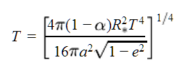
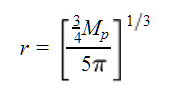
This section describes the algorithm that estimates the semimajor axis and planetary radius, if needed. Inputs to this routine include the planetary albedo α (assumed to be 0.2), eccentricity, tidal quality factor Qp (assumed to be 1000000), semiamplitude of the radial velocity K, period, stellar mass, effective temperature, stellar radius, and relative orbital inclination factor sin i=1.
- Get the planet mass m sin i >1 from the radial velocity K by iteration, until q > 1:
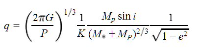
where G is Newton's constant, P is the period, K is the radial velocity semiamplitude, Mp is the planet mass, M* is the stellar mass, and e is the eccentricity (see, e.g., Kane 2007 Eq. 2). Since the algorithm assumes sin i = 1, this gives Mp directly. - Compute the semi-major axis, a,
- Compute the effective temperature,
- Compute the radius estimate by interpolating over a table of model parameters containing planet temperature and density information, returning a fiducial radius if necessary.
Transit Visibility
- For ground-based observatories: A transit is considered observable and reported in the output table if:
- The altitude of the Sun is below the twilight altitude threshold (-6°, -12°, or -18°, corresponding to civil, nautical, and astronomical twilight respectively, as selected in the web user interface); and
- The target is above the input altitude limit (or below the input airmass limit) at the time of the predicted transit midpoint, at the location of the selected observatory.
- For space-based observatories (currently JWST): A transit is considered observable if the midpoint falls within a window of target observability for the given telescope. Calculation of the observability windows for JWST take into account the pointing constraints (Sun and Earth) and spacecraft orbital position to find the date range that any location on the sky can be observed.
- For predictions independent of observer location: When the user requests predictions that are independent of observer location, visibility considerations are simply ignored, and the service returns either the next transit for a given system, or all transits that will occur within the requested observing window (depending on which option the user has selected).
For this purpose, the altitude of the sun is determined using the solar position algorithm of Reda & Andreas (2004).
Rise/Set Times
For ground-based observations (only), target rise, target set, and twilight times are calculated for the night of each observable transit as follows:
Target Rise and Target Set
- The positive and negative local hour angle limits at which the target rises above at sets below the requested altitude limit are calculated.
- The planet transit midpoint time (JD UT) is converted to Greenwich Mean Sidereal Time (GMST), following Meeus, 1998.
- The nearest GMST at which the host star transits the observer's local meridian (local hour angle = 0) is calculated.
- The GMST at rise and set are determined by calculating the GMST of the nearest passage of the target across the local hour angle limits to the local meridian passage (i.e., those immediately before and after the local meridian passage.)
- These are converted back to JD UT to give the target rise and set times.
- If a target never reaches below the altitude limit—i.e., if it is circumpolar—then a null value is returned. (Note that stars that never rise above the altitude limit will already have been filtered since their planet transit midpoints will never be observable.)
Note: We do not currently precess stellar coordinates to the epoch of the predicted transit. This can translate to systematic errors in rise/set times on the order of ~1min per decade between the epoch of the transit and the epoch of the coordinates.
Evening Twilight End and Morning Twilight Start
The sun's right ascension and declination at the time of transit midpoint are computed using an adaptation of the sunpos routine from the NASA IDL Astronomy User's Library. The same method is then applied as for calculating target rise and set, with some small differences, as follows:
- Find the nearest meridian anti-transit of the sun to the planet transit midpoint, in GMST (i.e., find the nearest local midnight).
- Find the nearest set and rise time of the sun below/above the chosen twilight altitude limit (-6°, -12°, or -18°) to the local midnight, in GMST.
- Convert the set/rise times to JD UT.
This approach avoids 24-hour wrapping errors due to precision limitations when the planet transit-midpoint is very close to the end of evening twilight or start of morning twilight.
Note: that the proper motion of the Sun during the course of the night is not currently accounted for. This leads to uncertainties of up ~2-4min in the twilight start/end times.
Observability Start and Observability End
The observability start and end columns in the output table give the start and end of the intersection of the period the target is up and the period the sky is dark (i.e., between twilights). This gives the best estimate of the full window during which the target can be observed on the night of a given planet transit event.
For calculations where the user has requested predictions for a non-zero orbital phase (secondary eclipse, quadratures, or custom phase), the time of the respective orbital phase is substituted for the planet transit midpoint.
UT calendar dates equivalents are made available for all JD time/date columns. Date conversion between Julian and calendar systems follow Murray & Dermott (1999).
Observability Statistics
Several additional useful quantities are calculated to aid in planning transit observations. These include:
| Duration of Target Observability | The difference between observability end and observability start times. |
| Duration Observable Before Event | The difference between event ingress time (without uncertainty padding) and observability start time. |
| Duration Observable After Event | The difference between observability end time and event egress (without uncertainty padding) |
| Duration Observable Outside Event | The sum of the observable durations before and after the transit (or eclipse) event |
| Event Fraction Observable | The ratio of the observable duration inside transit (or eclipse) to the transit duration. |
| Observable Baseline/Event Duration | The ratio of the observable duration outside the transit to the transit duration. This is useful if a significant number of observations are wanted outside transit in order, for example, to account for stellar variability, or to establish a good baseline against which to measure the transit depth. |
Transit Depth
In addition to providing a column in the output table which mirrors the Archive value (Transit Depth - Measured), a second column provides a calculated value, where possible, for use in the event that an explicit measured value is not available. Provided Rp the planet radius, and R*, the radius of the host star, are both available, the depth is calculated as:
Where δcalc is the calculated transit depth, Rp is the planet radius, and R* is the radius of the host star. This quantity is made available in the column labeled Transit Depth - Calculated.
«Previous Refining Transit Settings Definitions of Transit Parameters Next »
Last updated: 15 January 2020